Module 3: Spectroscopic Properties Calculation
Figure 1 shows the module designed for the spectroscopic properties calculations, such as experimental and theoretical intensity parameters, energy transfer rates, and the overall emission quantum yield.
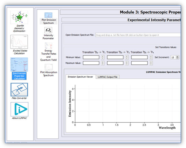
Figure 1. Module designed for the spectroscopic properties calculations.
The goal of the theoretical protocol consists mainly in calculating the emission quantum yield. For this reason, the module designed for the spectroscopic properties calculations was arranged in the following four sub modules:
i) In the first one, the experimental intensity parameters (Ωλ) are determined by the experimental emission spectrum;
ii) In the second one, the theoretical intensity parameters are calculated. These quantities are determined by the procedure of adjusting the charge factors and polarizabilities to reproduce the experimental intensity parameters.
iii) In the third one, the theoretical intensity parameters, together with the singlet and triplet excited state energies, are used to calculate the energy transfer rates. If the experimental lifetime of the 5D0 → 7F2 transition can also be provided, then, the emission quantum yield will be also theoretically quantified.
iv) And, in the fourth one, the theoretical absorption spectrum from the ORCA output file is produced;
In the next sections, we will now show how to calculate all these quantities using the LUMPAC program.
1. Experimental Intensity Parameters Calculation
Warming: To apply this module to calculate the experimental intensity parameters is mandatory to use a file obtained by experimentally measured emission spectrum. This file must be provided by you.
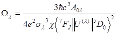
The experimental intensity parameters are determined through the following equation:
 Eq.
(1)
Eq.
(1)
where
the factor![]() is known as the Lorentz
local field correction term. The refractive index, n, has been assumed to
be equal to 1.5. The quantities <7F2||U(2)||5D0>2
= 0.0032, and <7F4||U(4)||5D0>2
= 0.0023 correspond to the squared reduced
matrix element. The term A01 is
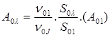
calculated by Eq. (2), while the quantities A02 and A04
are given by Eq. (3).
is known as the Lorentz
local field correction term. The refractive index, n, has been assumed to
be equal to 1.5. The quantities <7F2||U(2)||5D0>2
= 0.0032, and <7F4||U(4)||5D0>2
= 0.0023 correspond to the squared reduced
matrix element. The term A01 is
calculated by Eq. (2), while the quantities A02 and A04
are given by Eq. (3).
![]() Eq.
(2)
Eq.
(2)
 Eq.
(3)
Eq.
(3)
Parameters S01 and S0λ are the area under the spectrum peaks corresponding to the 5D0 → 7F1 and 5D0 → 7Fλ transitions, respectively. The quantities ν01 and ν0λ are the energy barycenters of the 5D0 → 7F1 and 5D0 → 7Fλ transitions, respectively. For europium (III), the 5D0 → 7F1 transition is assumed as a reference transition, because it is allowed by the magnetic dipole mechanism. Consequently, this transition does not practically depend on the characteristics of chemical environment, which changes from complex to complex.
The experimental intensity parameters are calculated by LUMPAC from the experimental emission spectrum. To do this, it is necessary to define the spectral areas related to the 5D0 → 7F1, 5D0 → 7F2 and 5D0 → 7F4 transitions. LUMPAC enables the selection of these areas by the user in an interactive manner.
Warming: Since the emission spectrum of Eu(DSACAC)3phen is not available, we decided to use a typical spectrum of an europium complex just to show the functionalities of this module. For this reason, in Section 3, the experimental intensity parameters here calculated will not be used as reference to compute the theoretical intensity parameters. Instead, we will use those from the article of Liang and Fang.
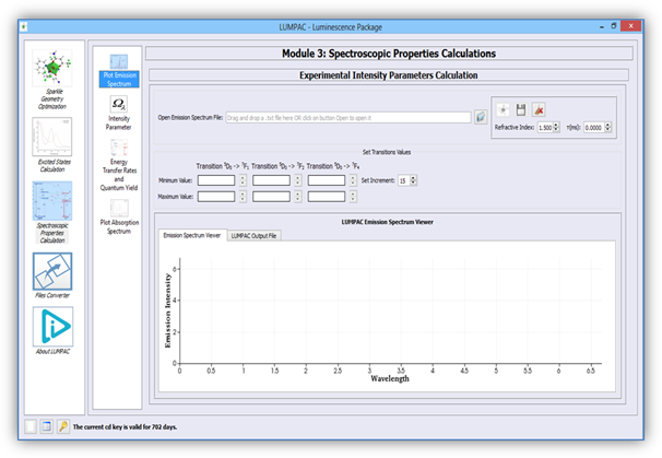
Figure 2. Module designed to calculate experimentally the intensity parameters, and radiative emission rate of a europium containing system.
Procedure for the Calculations of Intensity Parameters and
Radiative Emission Rate with LUMPAC
1.
Click on button ![]() (Figure 3) to open the .txt file of the emission file containing the
wavelengths versus emission intensities. These quantities must be separated either
by a comma (“,”) or by a blank space (“ ”) in the text file;
(Figure 3) to open the .txt file of the emission file containing the
wavelengths versus emission intensities. These quantities must be separated either
by a comma (“,”) or by a blank space (“ ”) in the text file;
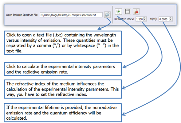
Figure 3. LUMPAC interface showing how to perform the experimental intensity parameters and experimental radiative emission rate calculations.
2. The areas related to the 5D0 → 7F1, 5D0 → 7F2, and 5D0 → 7F4 transitions must be adequately chosen by using the LUMPAC interface (Figure 4);
Using the UpDownArrows ![]() select the wavelength range under each of
the main peaks of the emission spectrum so that LUMPAC can integrate the
respective areas.
select the wavelength range under each of
the main peaks of the emission spectrum so that LUMPAC can integrate the
respective areas.
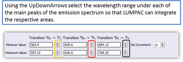
Figure 4. LUMPAC interface showing how to select each area under the main transition for europium systems
For example, for the 5D0 → 7F1 transition, use the orange updown arrows (circled in orange in Fig. 4). Be sure to select all three spectral ranges, as in the figure below. As you choose the wavelength ranges, the areas under the curves will be painted, as shown in Fig. 5.
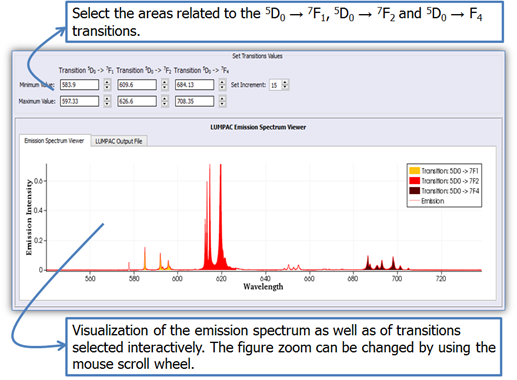
Figure 5. Emission spectrum viewer. The areas related to the 5D0 → 7F1, 5D0 → 7F2, and 5D0 → 7F4 transitions are highlighted.
3.
Button ![]() (Figure 3) will be enabled as soon as the .txt file is loaded; click
on it to perform the calculations of the experimental intensity parameters and
the experimental radiative emission rate.
(Figure 3) will be enabled as soon as the .txt file is loaded; click
on it to perform the calculations of the experimental intensity parameters and
the experimental radiative emission rate.
4. The non-radiative emission rate and the quantum efficiency will be calculated if the experimental lifetime is provided (Figure 3);
2. Theoretical Calculation of the Intensity Parameters
Figure 6 shows the LUMPAC module designed for the theoretical
calculation of the intensity parameters. By employing a non-linear algorithm, the
charge factors (g), and the polarizabilities (α), used in ![]() and
and ![]() calculations respectively, are
adjusted in order to reproduce the experimental values of Ω2
and Ω4. Section of Theory should be consulted for more
details.
calculations respectively, are
adjusted in order to reproduce the experimental values of Ω2
and Ω4. Section of Theory should be consulted for more
details.
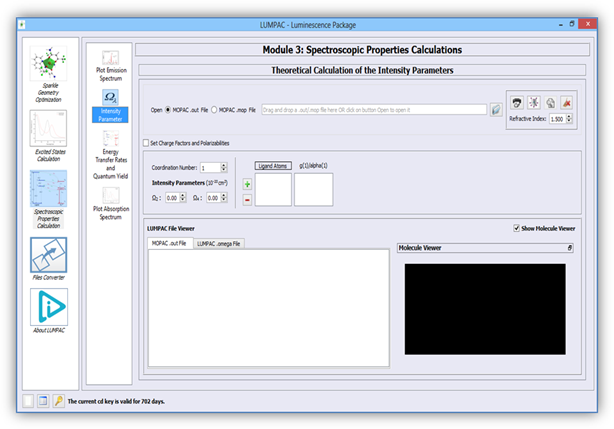
Figure 6. LUMPAC interface designed for the theoretical calculation of the intensity parameters.
Procedure for the Theoretical Calculation of the Intensity Parameters using LUMPAC
1.
Click on button ![]() (Figure 6) to open the MOPAC output file (.out) which contains
either the optimized geometry, or the starting structure (.mop). The option
“Open Mopac .mop File” enables the calculation of intensity parameters from
crystallographic data. For this purpose, the MOPAC input file (.mop) must be
created from these crystallographic coordinates.
(Figure 6) to open the MOPAC output file (.out) which contains
either the optimized geometry, or the starting structure (.mop). The option
“Open Mopac .mop File” enables the calculation of intensity parameters from
crystallographic data. For this purpose, the MOPAC input file (.mop) must be
created from these crystallographic coordinates.
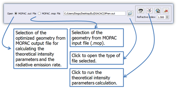
Figure 7. LUMPAC interface showing how to calculate theoretically the intensity parameters.
Figure 7 shows the different types of quantities that can be added to the printing of the intensity parameters allowed by LUMPAC.
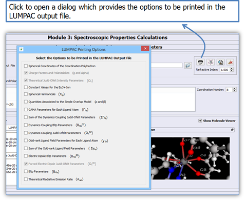
Figure 8. LUMPAC interface showing the different types of quantities that can be added to the printing of the intensity parameters allowed by LUMPAC.
2. Define the coordination number (Figure 9) in order to show the ligand atom labels in the molecule viewer (Figure 10).
3. Each ligand atom contains a value of g and α. However, atom groups with the same chemical environment must have the same g and α. LUMPAC enables a simple manner to specify the atom groups that have the same chemical environment (Figure 9);
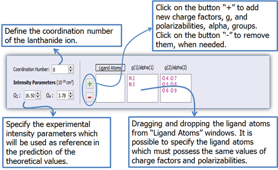
Figure 9. LUMPAC interface showing how to define the charge factors and polarizabilities groups related to the ligand atoms.
The following atoms are included in the same group (Figure 9) for the Eu(DSACAC)3(phen) system: N2 and N3 (phenanthroline nitrogen); O4, O5, O6, O7, O8 and O9 (beta-diketonate oxygen). It is only necessary to drag and drop each ligand atom in its respective group.
4. The values of Ω2 and Ω4 obtained by Liang and Xie for the Eu(DSACAC)3phen were 16.50 × 10⁻² cm2and 3.78 × 10⁻²⁰cm2 [1], respectively. After defining the g and α groups; set the experimental intensity parameters as shown in Fig. 9.
5.
Click on button ![]() (Figure 7) to perform the calculation of the intensity parameters. The
file containing the theoretical intensity parameters will be saved in
the same directory and have the same filename as the corresponding .out, but
with extension .omega.
(Figure 7) to perform the calculation of the intensity parameters. The
file containing the theoretical intensity parameters will be saved in
the same directory and have the same filename as the corresponding .out, but
with extension .omega.
Figure 10 shows the molecule viewer, emphasizing the atoms of the first coordination sphere of the europium ion. The ligand atoms coordinated to the lanthanide ion will be used to calculate the intensity parameters.
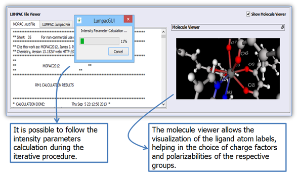
Figure 10. Molecule viewer showing the ligand atom labels for facilitating the selection of the respective charge factor and polarizability groups of the ligand atoms.
The radiative emission rate depends on Ω6, which is not experimentally measured. Because of that, the calculation of the intensity parameters is very important. By using theoretical calculations, the contribution from coupling dynamics (Ωd.c.λ), and from electric dipole (Ωe.d.λ) are determined, and this last one is used to predict the energy transfer rates via the multipolar mechanism. Section of Theory should be consulted for more details.
6. If the user already has values for the charge factors and polarizabilities, it is possible to calculate the intensity parameters directly (Figure 11);
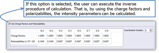
Figure 11. LUMPAC interface showing how to calculate the intensity parameters from the charge factors and polarizabilities.
3. Energy Transfer Rate and Emission Quantum Yield Calculations
Figure 12 shows the module designed for the energy transfer rate calculation and, if the experimental lifetime is provided, for the quantum efficiency and the overall emission quantum yield calculation. All these quantities can be calculated by using the theoretically calculated intensity parameters according to the procedure described in 2, together with the ORCA output file created in Module 2.
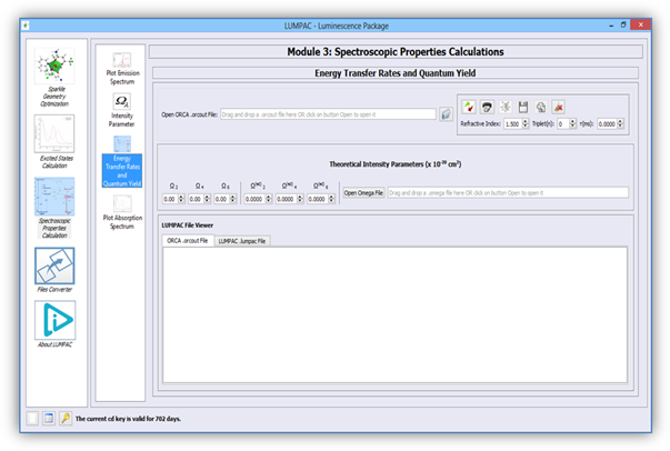
Figure 12. Module designed for the energy transfer rates and emission quantum yield calculations.
Procedure for Energy Transfer Rates and Emission Quantum Yield Calculations using LUMPAC
1.
Click on button ![]() (Figure 12) to open the ORCA output file (.orcout) calculated by the
procedure described in Module 2;
(Figure 12) to open the ORCA output file (.orcout) calculated by the
procedure described in Module 2;
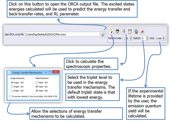
Figure 12. LUMPAC interface showing how to determinate the energy transfer rates, and the emission quantum yield from the ORCA output file.
2. As soon as the .orcout is loaded, the .omega file containing the intensity parameters calculated by the procedure described in Section 2 (Figure 13) will be loaded automatically. Therefore, it must be in the same directory and with the same filename as the corresponding .orcout, but with .omega extension. If the .omega file is not loaded automatically, provide manually the values of the calculated intensity parameters by using the LUMPAC interface, or setting the corresponding .omega file.
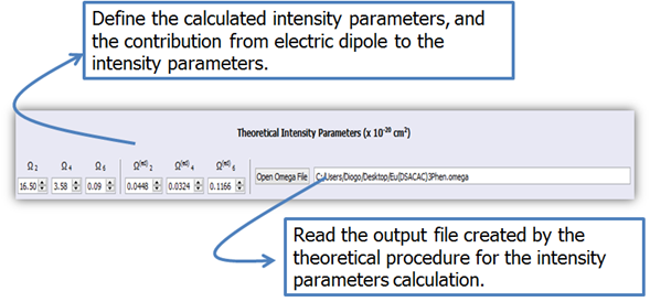
Figure 13. LUMPAC interface showing how to specify the intensity parameters used to calculate the energy transfer rate and emission quantum yield.
3.
Click on button ![]() (Figure 12) if you want to set the used energy transfer channels for
systems containing europium ion;
(Figure 12) if you want to set the used energy transfer channels for
systems containing europium ion;
The energy transfer (WET) and back-transfer (WBT) rates between the ligands and the lanthanide ion are calculated by the model based on the 4f – 4f transitions, developed by prof. Malta. As can be seen in Figure 12 the energy transfer channels can be easily changed. The resonance of the excited states of the ligands with the excited states of the lanthanide ion is the criterion to be applied in order to decide which channels to use.
4.
Click on button ![]() (Fig. 12) if you want to print other quantities that were used to
perform the energy transfer rates. When the button
(Fig. 12) if you want to print other quantities that were used to
perform the energy transfer rates. When the button![]() is clicked, a dialog like shown in Fig. 14 will appear.
is clicked, a dialog like shown in Fig. 14 will appear.
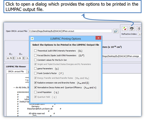
Figure 14. LUMPAC interface showing the quantities that can be printed by LUMPAC when the calculations of the energy transfer rates and yield quantum are performed
5.
Click on button ![]() (Figure
12) to perform energy transfer and back-transfer rates calculations. If the
experimental lifetime is provided, the overall emission quantum yield will be calculated;
(Figure
12) to perform energy transfer and back-transfer rates calculations. If the
experimental lifetime is provided, the overall emission quantum yield will be calculated;
6. The LUMPAC file viewer will display the results when the calculation is finished (Figure 15).
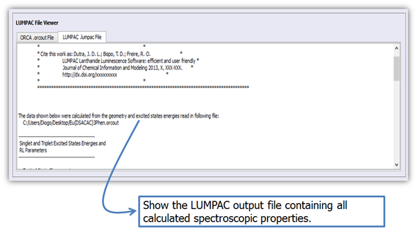
Figure 15. File viewer of LUMPAC showing its output file.
Figure 16 shows the LUMPAC output file containing all calculated spectroscopic properties.
|
********************************************************************************** |
|
LUMPAC - Lanthanide Luminescence Software - version 1.0 |
|
|
|
Cite this work as: Dutra, J. D. L.; Bispo, T. D.; Freire, R. O. |
|
LUMPAC Lanthanide Luminescence Software: efficient and user friendly |
|
Journal of Chemical Information and Modeling 2013, X, XXX-XXX. |
|
http://dx.doi.org/xxxxxxxxx |
|
********************************************************************************** |
|
|
|
The data shown below were calculated from the geometry and excited states energies read in following file: |
|
C:/Users/Diogo/Desktop/Eu(DSACAC)3Phen.orcout |
|
|
|
------------------------------------------------------- |
|
Theoretical Judd-Ofelt Intensity Parameters, omega(l) |
|
------------------------------------------------------- |
|
|
|
omega(2) = 16.50e-20 cm^2 |
|
omega(4) = 3.78e-20 cm^2 |
|
omega(6) = 0.14e-20 cm^2 |
|
|
|
----------------------------------------------------------- |
|
Forced Electric Dipole Judd-Ofelt Parameters, omegaED (l) |
|
----------------------------------------------------------- |
|
|
|
omegaED(2) = 0.0625e-20 cm^2 |
|
omegaED(4) = 0.0958e-20 cm^2 |
|
omegaED(6) = 0.3947e-20 cm^2 |
|
|
|
----------------------------------- |
|
Constant values for the Eu3+ Ion |
|
----------------------------------- |
|
|
|
Used Racah Tensor Operator: <f|C(2)|f> = -1.3660 <f|C(4)|f> = 1.1280 <f|C(6)|f> = -1.2700 |
|
|
|
Used Shielding Factor: sigma(2) = 0.600 sigma(4) = 0.136 sigma(6) = 0.100 |
|
|
|
Radial Integrals: r(2) = 2.568e-17 cm^2 r(4) = 1.582e-33 cm^4 r(6) = 1.981e-49 cm^6 |
|
|
|
------------------------------------------------- |
|
Singlet and Triplet Excited States Energies and |
|
RL Parameters |
|
------------------------------------------------- |
|
|
|
Excited State Chosen = 1 |
|
RL Singlet: 5.0165 Angs Singlet Energy: 37613.10 cm^-1 |
|
RL Triplet: 5.5621 Angs Triplet Energy: 20931.60 cm^-1 |
|
|
|
RL: distance from the donor state located at the organic ligands |
|
and the Eu3+ ion nucleus. |
|
|
|
--------------------- |
|
gama(l) Parameters |
|
--------------------- |
|
|
|
gama(2) = 1.4722e+25 gama(4) = 4.6789e+22 gama(6) = 2.2309e+20 |
|
|
|
------------------------------------------------------ |
|
Frank Condon's Factor (F), this factor depend on the |
|
------------------------------------------------------ |
|
|
|
F (Singlet - 5D4) = 1.0077e+09 erg^-1 |
|
F (Triplet - 5D1) = 5.7813e+11 erg^-1 |
|
F (Triplet - 5D0) = 3.0544e+11 erg^-1 |
|
|
|
------------------------------------------------------ |
|
Energy Transfer (Wet) and Back-Transfer Rates (Wbt) |
|
Wet from the Multipolar Mechanism (WetMM) |
|
Wet from the Exchange Mechanism (WetEM) |
|
------------------------------------------------------ |
|
|
|
Energy Transfer Rates |
|
WetMM (Singlet -> 5D4) = 1.81e+02 s^-1 |
|
WetEX (Triplet -> 5D1) = 8.33e+09 s^-1 |
|
WetEX (Triplet -> 5D0) = 8.45e+09 s^-1 |
|
|
|
Energy Back-Transfer Rates |
|
WbtMM (Singlet -> 5D4) = 2.26e-19 s^-1 |
|
WbtEX (Triplet -> 5D1) = 1.08e+06 s^-1 |
|
WbtEX (Triplet -> 5D0) = 2.22e+02 s^-1 |
|
|
|
------------------------------------- |
|
Radiative emission rate (Arad) and |
|
Branchio Rates (beta) |
|
------------------------------------- |
|
|
|
Used Refractive Index = 1.500 |
|
|
|
Arad = 605.09 s^-1 |
|
|
|
Beta values (contribution of each 5D0 -> 7Fj transition in percentage to radiative decay rate) |
|
|
|
5D0 -> 7F1: 8.18 5D0 -> 7F2: 82.27 5D0 -> 7F3: 0.00 |
|
|
|
5D0 -> 7F4: 9.53 5D0 -> 7F5: 0.00 5D0 -> 7F6: 0.02 |
|
|
|
--------------------------------------- |
|
Nonradiative Decay Rates (Anrad) and |
|
Quantum Efficiency |
|
--------------------------------------- |
|
|
|
Used Experimental Lifetime = 0.6060 ms |
|
|
|
Anrad = 1045.07 s^-1 |
|
|
|
Quantum Efficiency = 36.67 % |
|
|
|
---------------------------------------------------------------------------- |
|
Level population of each State Involved in the Process of Energy Transfer |
|
---------------------------------------------------------------------------- |
|
|
|
Excited Singlet Population = 0.1428 |
|
Triplet Population = 0.0000 |
|
5D4 Population = 0.0000 |
|
5D1 Population = 0.0000 |
|
5D0 Population = 0.0005 |
|
7Fj Population = 0.8567 |
|
|
|
----------------------------- |
|
Quantum Yield: 36.30 % |
|
----------------------------- |
Figure 16. LUMPAC output file showing all calculated spectroscopic properties.
4. Theoretical Calculation of the Absorption Spectrum
Figure 17 shows the module designed for the theoretical calculation of the absorption spectrum from the file with extension .orcout created by the ORCA program.
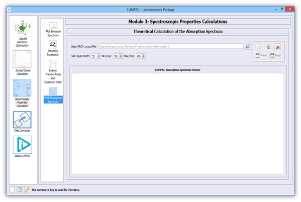
Figure 17. Module designed for the theoretical calculation of the absorption spectrum from file created by the ORCA program.
Procedure for Theoretical Calculation of the Absorption using LUMPAC
1.
Click on button ![]() (Figure 18) to open the ORCA output file (.orcout).
(Figure 18) to open the ORCA output file (.orcout).
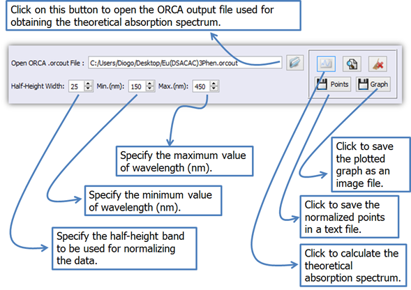
Figure 18. LUMPAC interface showing how to obtain the absorption spectrum from the ORCA output file.
Electronic transitions are allowed from the singlet ground state to singlet excited states, whose probability of occurrence is proportional to a quantity known as the oscillator strength, fosc, of the transition, as shown in Fig 19. The theoretical absorption spectrum is obtained by using the oscillator strength and the excitation energy and by using the typical half-height band of 25nm. LUMPAC will then produce an absorption spectrum. If you prefer, you can also modify either or both the half-height band and the wavelength range to other values, such as ones taken from experimental spectra.
|
. . . |
|||||||||||
|
------------------------------------------------------------------------------------------------------------------------ |
|||||||||||
|
ABSORPTION SPECTRUM VIA TRANSITION ELECTRIC DIPOLE MOMENTS |
|||||||||||
|
--------------------------------------------------------------------------------------------------------------- |
|||||||||||
|
State |
Energy |
Wavelength |
fosc |
T2 |
TX |
TY |
TZ |
||||
|
|
(cm-1) |
(nm) |
|
(au**2) |
(au) |
(au) |
(au) |
||||
|
--------------------------------------------------------------------------------------------------------------- |
|||||||||||
|
1 |
30387.8 |
329.1 |
0.752144505 |
8.14851 |
-2.04436 |
1.98244 |
-0.19760 |
||||
|
2 |
31400.6 |
318.5 |
0.701059939 |
7.35009 |
1.66818 |
0.02395 |
-2.13698 |
||||
|
3 |
32069.8 |
311.8 |
1.018622378 |
10.45666 |
-0.41608 |
3.20660 |
-0.03584 |
||||
|
. . . |
|||||||||||
|
48 |
32185.9 |
310.7 |
spin forbidden (mult=3) |
||||||||
|
49 |
32279.5 |
309.8 |
spin forbidden (mult=3) |
||||||||
|
50 |
32454.9 |
308.1 |
spin forbidden (mult=3) |
||||||||
|
. . . |
|||||||||||
Figure 19. A section of the .orcout file where the singlet energies, and the oscillator strengths of the singlet → singlet transitions are shown. These quantities are used to obtain the theoretical absorption spectrum.
2.
Click on button ![]() to
perform the calculation of the absorption spectrum, which will appear as below
(Fig. 20).
to
perform the calculation of the absorption spectrum, which will appear as below
(Fig. 20).
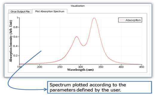
Figure 20. LUMPAC interface showing the absorption spectrum created by LUMPAC.
LUMPAC will then produce a publication quality .jpg image of the spectrum, which can be saved, as well as a .txt file with the raw data and oscillator strengths which can also be saved either an image file, or as a .txt file.
Bibliographic References