Theory

Theoretical Foundations of the Models Implemented in LUMPAC

Process of Geometry Optimization

The potential energy surface (PES) consists of a surface of the calculated energy ( $E$ ) as a function of the geometric parameters of a molecule (q), $E = f(q_1, q_2, ..., q_n)$ , where n is the number of geometric parameters. A steady point in the PES is defined by a flat point on the surface, being mathematically represented by $dE/dq=0$ . If ${{d}^{2}}E/d{{q}^{2}}<0$ , the steady point is a transition state. In contrast, if ${{d}^{2}}E/d{{q}^{2}}>0$ , the steady point corresponds to a minimum of energy, usually a local minimum. The lowest of the local minima, the global minima, usually defines the most stable ground state geometry of the molecule.

In general, the geometry optimization procedure consists in supplying an input molecular structure with geometrical parameters $q_0$ hoped to be as close as possible to the steady point desired. This reasonable geometry is then submitted to an algorithm which systematically alters the atomic positions until a minimum steady point is reached, defined by its geometric parameters $q_i$ .

The computational chemistry methods that are applied to perform geometry optimizations may be divided roughly into two groups: molecular mechanics methods and quantum methods. In molecular mechanics methods, roughly speaking, the molecule is treated as set points, each representing an atom, interconnected by springs, representing the chemical bonds. Such methods are very fast because the potentials are classic and no electronic wave functions are present. In contrast, quantum methods attempt to solve, for the entire molecular system, the famous Schrödinger eigenvalue equation $H\psi =E\psi$ , where $H$ is the Hamiltonian operator, $\psi$ is the wave function (the eigenvector), and E is the total energy of the system (the eigenvalue).

The quantum computational methods are usually divided into four groups: i) the Hartree-Fock methods which solve the self-consistent field Schrödinger equation under the independent particle approximation, calculating all possible two-electron integrals; ii) the post Hartree-Fock methods, which also take into consideration the contributions due to electron correlations; iii) the semiempirical quantum chemical methods, which are based on the Hartree-Fock method, though some integrals are replaced by parameters, adjusted to reproduce experimental data during its process of development; and, finally, iv) the methods based on density functional theory (DFT), which consider the electron density as the fundamental entity, and not the wave function as all other quantum methods do.

The method of choice for performing geometry optimizations depends mainly on the number of atoms present in the desired system.

Normally, the standard procedure for geometry optimization consists in building the chemical structure by adding atoms in arbitrary positions and by subsequently connecting them according to their chemical bonds. The next step is to previously optimize the geometry by using less costly computational methods. Molecular mechanics methods are quite fast methods and some of them have parameters available for almost all elements. As a result, although molecular mechanics methods do not provide accurate geometries, such methods are usually applied to transform the drawn geometries into reasonably good starting structures for refinement by computationally more accurate and usually more expensive calculations [1].

The ground state geometries of lanthanide complexes can be calculated by two different quantum chemical based approaches: i) DFT or ab initio methods with effective core potentials (ECP) for treating the lanthanide ions, or ii) semiempirical methods. In 2006 [2] and 2011 [3] two papers were published in order to compare geometries predicted by semiempirical methods with those predicted by ab initio and DFT methods, with crystallographic data as reference. In contrast to what would be expected, the results showed that by enlarging the size of the basis set, or by including electron correlation, or both, deviations of the predicted coordination polyhedrons with respect to the crystallographic ones consistently increased, reducing the quality of the results. And among all ab initio methods evaluated, the method RHF/STO-3G using the MWB core effective potential was the most efficient for predicting the coordination polyhedron of lanthanide complexes [2]. This result confirms that the Sparkle models, which demand a much lower computational effort, have higher accuracy in calculations and modeling, when compared to ab initio/ECP ones [3].

In LUMPAC, the Sparkle models will be used in the geometry optimization step because such methods have an excellent capability of geometry prediction and also a considerably low computational cost. As a result, we will now provide a detailed description of these models. The procedure of development of the Sparkle model consists in parameterizing a semiempirical Hamiltonian, such as AM1 or PM3, for example, in which the lanthanide ion is replaced by a +3e point charge. This point charge is subjected to a repulsive potential $exp(-\alpha r)$ , where the parameter $\alpha$ quantifies the size of the ion. This mathematic entity is called “sparkle”. As the bond between Ln³⁺ and atom ligands has high ionic character, the Sparkle model has been consistently proven to be adequate.

The first Sparkle model, named SMLC (Sparkle Model for the Calculation of Lanthanide Complexes), was developed by Andrade and coworkers in 1994 [4]. This version was parameterized for the AM1 semiempirical model with only one experimental structure in the parameterization set: the tris(acetylacetonate)-(1,10-phenanthroline) of europium (III). When this Sparkle model version was evaluated for a representative test containing 96 europium complexes, the SMLC model lead to errors of approximately 0.68 $\AA$ for Ln $-$ L, lanthanide $-$ ligand atom, distances. However, the second parameterized version of the Sparkle model [5], SMLC II, published in 2004, included Gaussian functions in the core-core repulsion energy. The errors for Ln–L distances decreased from 0.68 to 0.28 $\AA$ when tested with the same europium structures set.

A new and much more sophisticated parameterization scheme was then carried out within AM1 for the Sparkle model in 2005 and was initially developed for Eu³⁺, Gd³⁺, and Tb³⁺[6]. This new version of the model was called Sparkle/AM1. The main changes consisted in the application of more sophisticated statistical techniques, both in the selection of the most representative training sets as well as in the validation of the parameters obtained. In the Sparkle/AM1 model development of the three parameterized ions, more than 200 different crystallographic structures were used together with a new response function for minimization in the parameterization procedure. These changes made it possible to decrease the errors for Ln–L distances from 0.28 to 0.09 $\AA$ in europium complexes. Test sets of gadolinium complexes (70 structures) and of terbium complexes indicated errors of approximately 0.07 $\AA$ . Then, the Sparkle/AM1 model was generalized for all types of ligands and parameterized for all 15 trivalent lanthanide ions [7-14]. Currently, the Sparkle models are also parameterized for the following semiempirical models: PM3 [15-21], PM6 [22], PM7 [23] and RM1 [24].

The geometry optimization of lanthanide complexes has a great importance for studying the luminescent properties of the system. All published Sparkle models (Sparkle/AM1, Sparkle/PM3, Sparkle/PM6, Sparkle/PM7 and Sparkle/RM1) are available in MOPAC2012 [25]. The choice of which of the available Sparkle models is to be used must be based mainly on the capability of the underlying semiempirical method, either AM1, PM3, PM6, RM1 or PM7 to correctly describe the specific ligands involved. Nevertheless, many tests performed by our group suggest Sparkle/RM1 to be the version that presents the best overall results.

Excited States Calculation

The singlet and triplet excited states of the organic part can be calculated by using methods based on time-dependent density functional theory (TD-DFT) [26] or by the semiempirical INDO/S method [27, 28]. In 2001, Gorelsky and Lever [36] compared these two methodologies for the ground and excited states calculations of Ru(II) complexes. The electronic spectra obtained by these two different methods showed excellent agreement with each other. However, even today, the TD-DFT method is still inappropriate to treat complexes with more than 100 atoms, due to its high demand of computational resources.

Santos and coworkers evaluated the accuracy of the semiempirical INDO/S method in comparison with TD-DFT ab initio results in studies of lanthanide complexes [29]. The results showed that triplet state energies calculated by the semiempirical method presented errors similar to those obtained by TD-DFT methodology, with the advantage of being hundreds of times faster.

In this context, the geometries optimized by the Sparkle models are used to calculate the singlet and triplet excited states by using the configuration interaction simple (CIS) of INDO/S, which has an accuracy of about 1000 cm^-1 [27, 28]. This method is implemented in ZINDO [30] and ORCA [31] programs. In this procedure, a point of charge +3e represents the lanthanide ion [32].

Intensity Parameters Calculation

The intensity parameters, $\Omega_\lambda$ ( $\lambda$ = 2, 4, and 6), are calculated by Judd-Ofelt theory [33, 34]. According to this theory, the central ion is affected by the nearest neighbor atoms, through a static electric field also referred as crystal or ligand field. Judd and Ofelt described, in independent works, the importance of the electric dipole mechanism for the 4f $-$ 4f transitions from the mixing of a ground state 4f^N configuration with excited state configurations of opposite parity through the odd terms of the ligand field Hamiltonian. All 4f orbitals have the same parity, that is ${{\left( -1 \right)}^{l}}$ , where $l$ = 3 for lanthanide ions. Then, the mixing are between the 4f orbitals plus higher-n orbitals, such as the 5d orbital, which presents $l$ = 2, and has an opposite parity to that of the f orbital.

The intensity parameters describe the interaction between the lanthanide and ligand atoms, and are calculated by Eq. ( $\ref{eq:omega}$ ).

{{\Omega }_{\lambda }}=(2\lambda +1)\sum\limits_{t=\lambda -1}^{\lambda +1(odd)}{\sum\limits_{p=-t}^{t(all)}{\frac{{{\left| {{B}_{\lambda tp}} \right|}^{2}}}{(2t+1)}}} \label{eq:omega}

One aspect which is very important for the possible application of this theory is to know the values that each of the rank variables $\lambda$ , $t$ , and $p$ may assume in relation to each other. As can been seen in Eq. ( $\ref{eq:omega}$ ), for example, when $\lambda$ is equal to 2, $t$ will be equal to 1 and 3, whereas the values of $p$ will be equal to 0, 1, ..., $t$ .

The $B_{\lambda t p}$ parameters are calculated by:

{{B}_{\lambda tp}}=B_{\lambda tp}^{ed}+B_{\lambda tp}^{dc} \label{eq:bltp}

The first term, $B_{\lambda tp}^{ed}$ , refers only to the forced electric dipole (ED) contribution, and are given by Eq. ( $\ref{eq:bltp_ed}$ ).

B_{\lambda tp}^{ed}=\frac{2}{\Delta E}\left\langle {{r}^{t+1}} \right\rangle \theta (t,\lambda )\gamma _{p}^{t} \label{eq:bltp_ed}

The term $\Delta E$ corresponds to the difference of energy between the ground state barycenters and the first excited state configuration of opposite parity. The radial integrals, $\left\langle {{r}^{\lambda }} \right\rangle$ , were taken from reference [35], with an extrapolation for the quantity $\left\langle {{r}^{8}} \right\rangle$ . The values of radial integrals for Eu³⁺ ion are $\left\langle {{r}^{2}} \right\rangle$ = 0.9175 a.u., $\left\langle {{r}^{4}} \right\rangle$ = 2.0200 a.u., $\left\langle {{r}^{6}} \right\rangle$ = 9.0390 a.u., and $\left\langle {{r}^{8}} \right\rangle$ = 110.0323 a.u. The terms $\theta(t,p)$ are numeric factors associated with each lanthanide ion and are estimated from radial integrals of Hartree-Fock calculations [36]. The values of $\theta(t,p)$ are $\theta(1,2) = -0.17$ ; $\theta(3,2) = 0.345$ ; $\theta(3,4) = 0.18$ ; $\theta(5,4) = -0.24$ ; $\theta(5,6) = -0.24$ , and $\theta(7,6) = 0.24$ , for Eu³⁺ ion [36].

The second term of Eq. ( $\ref{eq:bltp}$ ), $B_{\lambda tp}^{dc}$ , refers only to the dynamics coupling (DC) contribution and is given by Eq. ( $\ref{eq:bltpfull}$ ). This contribution is complementary to the one from the Judd-Ofelt static electric field model, and was firstly considered by Mason and coworkers [37]. The dynamics coupling mechanism, which is more important than the electric dipole mechanism for some transitions, is due to the high gradient of the electromagnetic field generated by the ligands when they interact with an incident external field. The DC mechanism depends on the nature of both ligands and on the coordination geometry, and explains the hipersensitivity in 4f $-$ 4f transitions [36].

B_{\lambda tp}^{dc}=-{{\left[ \frac{\left( \lambda +1 \right)\left( 2\lambda +3 \right)}{2\lambda +1} \right]}^{1/2}}\left\langle {{r}^{_{\lambda }}} \right\rangle (1-{{\sigma }_{\lambda }})\left\langle f\left\| {{C}^{\left( \lambda \right)}} \right\|f \right\rangle \Gamma _{p}^{t}{{\delta }_{t,\lambda +1}} \label{eq:bltpfull}

The quantity $(1 – \sigma_\lambda)$ is a shielding field due to 5s and 5p filled orbitals of lanthanide ions, which have a radial extension larger than those of the 4f orbitals [36]. The values of $\sigma_\lambda$ are $\sigma_2 =$ 0.600, $\sigma_4 =$ 0.139 and $\sigma_4 =$ 0.100. $\left\langle f\left\| {{C}^{\left( \lambda \right)}} \right\|f \right\rangle$ is a tensor operator of rank $\lambda$ ( $\lambda$ = 2, 4, and 6) with values $\left\langle 3\left\| {{C}^{\left( 2 \right)}} \right\|3 \right\rangle$ = -1.366, $\left\langle 3\left\| {{C}^{\left( 4 \right)}} \right\|3 \right\rangle$ = 1.128, and $\left\langle 3\left\| {{C}^{\left( 6 \right)}} \right\|3 \right\rangle$ = -1.270 for lanthanide ions. ${{\delta }_{t,\lambda +1}}$ is the Kronecker delta function. As such, $B_{\lambda tp}^{dc}$ is equal to 0 when $t$ is different from the $\lambda + 1$ .

The parameters $\gamma _{p}^{t}$ ( $t$ = 1, 3, 5, and 7), given by Eq. ( $\ref{eq:gamma_tp}$ ), are the so-called odd-rank ligand field parameters and contains a sum over the surrounding atoms.

\gamma _{p}^{t}={{\left( \frac{4\pi }{2t+1} \right)}^{{}^{1}/{}_{2}}}{{e}^{2}}\sum\limits_{j}{{{\rho }_{j}}{{\left( 2{{\beta }_{j}} \right)}^{t+1}}\frac{{{g}_{j}}}{R_{j}^{t+1}}Y_{p}^{t*}\left( {{\theta }_{j}},{{\phi }_{j}} \right)} \label{eq:gamma_tp}

$Y_{p}^{t*}\left( {{\theta }_{j}},{{\phi }_{j}} \right)$ are the conjugated spherical harmonics. As can be observed in Eq. ( $\ref{eq:gamma_tp}$ ), the spherical harmonics depend on the spherical coordinates $\left( {{\theta }_{j}},{{\phi }_{j}} \right)$ of the j ligand atoms.

The term ${{\rho }_{j}}{{\left( 2{{\beta }_{j}} \right)}^{t+1}}$ present in Eq. ( $\ref{eq:gamma_tp}$ ) according to the Simple Overlap Model (SOM) [38, 39] developed by prof. Oscar Malta (UFPE, Brazil), formalizes that crystal field Hamiltonian and is adequately calculated as a function of the charge density $\left( -ge\rho \right)$ between the lanthanide ion and the $j$ ligand atoms.

The SOM model assumes two postulates [38]: i) the 4f energy potential is generated by charges, uniformly distributed in a small region located around the mid-points of the lanthanide–ligand chemical bonds; and ii) the total charge in each region is equals to $-ge\rho$ , where the $\rho$ parameter is proportional to the magnitude of the total overlap between the lanthanide ion and the ligand atoms. Figure 1 shows a sketch of the effective charges for a hypothetical complex (LnL₃). The vector ${{\vec{R}}_{j}}$ represents the position of the $j$ ligand atoms, and the vector ${{\vec{r}}_{j}}$ represents the position of the $i^{th}$ electron of the central metal ion.

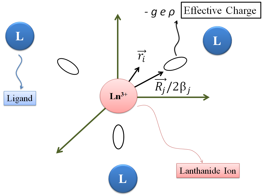
Figure 1. Graphical representation of the Simple Overlap Model.

In other words, the term ${{\rho }_{j}}{{\left( 2{{\beta }_{j}} \right)}^{t+1}}$ introduces a correction to the crystal field parameters of the point charge electrostatic model (PCEM), $\gamma _{p}^{t}\left( PCEM \right)$ , such that $\gamma _{p}^{t}\left( PCEM \right)={{\rho }_{j}}{{\left( 2{{\beta }_{j}} \right)}^{t+1}}\gamma _{p}^{t}\left( SOM \right)$ . This way, this correction confers a degree of covalency to the point charge model from the inclusion of the parameter $\rho$ , since PCEM treats the metal-ligand atom bonds as a purely electrostatic phenomenon.

The effective charges are assumed to be at positions defined at the distances given by ${{\vec{R}}_{j}}/2{{\beta }_{j}}$ . The factor $\beta_j$ , given by Eq. ( $\ref{eq:beta}$ ), indicates that the effective charges may not be exactly at ${{\vec{R}}_{j}}/2$ . The plus sign in Eq. ( $\ref{eq:beta}$ ) is used when the barycenter of the overlap region is displaced towards the ligand, which happens in the case of oxygen and fluorine coordinating atoms. The minus sign is used when this barycenter is displaced towards the central ion, as is the case of nitrogen and chlorine coordinating atoms.

{{\beta }_{j}}=\frac{1}{1\pm {{\rho }_{j}}} \label{eq:beta}

The overlap between 4f orbitals and the valence orbitals of the $j$ ligands, ${{\rho }_{j}}$ , is calculated by Eq. ( $\ref{eq:rho}$ ).

{{\rho}_{j}}={{\rho }_{0}}{{\left( \frac{{{R}_{0}}}{{{R}_{j}}} \right)}^{n}} \label{eq:rho}

where ${{\rho }_{0}}$ is a constant equal to 0.05 and $n$ is equal to 3.5 for the lanthanides. $R_0$ is the smallest among all lanthanide–ligand atom distances.

The parameters $\Gamma _{p}^{t}$ ( $t$ = 1, 3, 5, and 7), like the parameter $\gamma _{p}^{t}$ , also depends on the coordination geometry and on the chemical environment around the lanthanide ion, and is given by Eq. ( $\ref{eq:GAMMA1_tp}$ ).

\Gamma _{p}^{t}={{\left( \frac{4\pi }{2t+1} \right)}^{1/2}}\sum\limits_{j}{\frac{{{\alpha }_{j}}}{R_{j}^{t+1}}Y_{p}^{t*}\left( {{\theta }_{j}},{{\phi }_{j}} \right)} \label{eq:GAMMA1_tp}

The limitations in the intensity parameters calculation consist in determining the quantities, $\gamma _{p}^{t}$ and $\Gamma _{p}^{t}$ . As a result, it is necessary to use the experimental intensity parameters.

The charge factors and polarizabilities, used in $\gamma _{p}^{t}$ and $\Gamma _{p}^{t}$ calculations, respectively, are adjusted to reproduce the experimental intensity parameters. During the adjustment procedure, the intensity parameters calculated ( $\Omega _{\lambda }^{calc}$ ) from the optimized geometry, obtained from Sparkle model, are compared with the experimental intensity parameters ( $\Omega _{\lambda }^{\exp }$ ). The response function ( $F_{resp}$ ) is defined by Eq. ( $\ref{eq:fresp}$ ).

{{F}_{resp}}={{(\Omega _{2}^{calc}-\Omega _{2}^{\exp })}^{2}}+{{(\Omega _{4}^{calc}-\Omega _{4}^{\exp })}^{2}} \label{eq:fresp}

Emission Radiative Rate Calculation

The emission radiative rate ( $A_{rad}$ ), taking into account the magnetic dipole and forced electric dipole mechanisms, is given by Eq. ( $\ref{eq:arad}$ ):

A({}^{5}{{D}_{0}}-{}^{7}{{F}_{J}})=\frac{64{{\pi }^{4}}{{v}^{3}}}{3h(2J+1)}\left[ \frac{n{{({{n}^{2}}+2)}^{2}}}{9}{{S}_{ed}}+{{n}^{3}}{{S}_{md}} \right] \label{eq:arad}

where $\Delta E$ is the difference of energy between the ⁵D₀ and ⁷F_J states (in cm^-1), $h$ is the Planck constant, $2J + 1$ is the degeneracy of the initial state, and $n$ is the refractive index of the medium, usually assumed to be equal to 1.5. $S_{ed}$ (Eq. ( $\ref{eq:sed}$ )) and $S_{md}$ in Eq. ( $\ref{eq:smd}$ ) are the magnetic dipole and forced electric dipole mechanisms, respectively.

{{S}_{ed}}={{e}^{2}}\sum\limits_{\lambda =2,4,6}{{{\Omega }_{\lambda }}{{\left| \left\langle {}^{5}{{D}_{0}}\left\| {{U}^{(\lambda )}} \right\|{}^{7}{{F}_{J}} \right\rangle \right|}^{2}}} \label{eq:sed}

The squared matrix elements ${{\left\langle {}^{5}{{D}_{0}}\left\| {{U}^{(2)}} \right\|{}^{7}{{F}_{2}} \right\rangle }^{2}}$ , ${{\left\langle {}^{5}{{D}_{0}}\left\| {{U}^{(4)}} \right\|{}^{7}{{F}_{4}} \right\rangle }^{2}}$ , and ${{\left\langle {}^{5}{{D}_{0}}\left\| {{U}^{(6)}} \right\|{}^{7}{{F}_{6}} \right\rangle }^{2}}$ are equal to 0.0032, 0.0023, and 0.0002, respectively, for Eu³⁺ [40].

{{S}_{md}}=\frac{{{\hbar }^{2}}}{4m{{c}^{2}}}{{\left\langle {J}'\left\| L+2S \right\|J \right\rangle }^{2}} \label{eq:smd}

where $m$ is the electron mass. The matrix elements that appear in Eq. ( $\ref{eq:smd}$ ) above are determined according to the intermediate coupling mechanism. The ⁵D₀ $\rightarrow$ ⁷F₁ transition is the only one that does not have contributions from the electric dipole mechanism and are quantified theoretically as $S_{md} = 9,6\times10^{-42}$ esu² cm² [41].

The ⁵D₀ $\rightarrow$ ⁷F_J transitions ( $J$ = 0, 3, and 5) are forbidden by magnetic dipole and forced electric dipole mechanisms, that is, their contributions are equal to 0.

The contributions of each transition to the emission radiative rate are calculated by Eq. ( $\ref{eq:beta0j}$ ), and are named branching ratios ( $\beta_{0,J}$ ).

{{\beta }_{0,J}}=\frac{{{A}_{0,J}}}{{{A}_{rad}}} \label{eq:beta0j}

Energy Transfer Rates Calculation

The theoretical model used to calculate the energy transfer rate between the organic ligands and the lanthanide ion was developed by Malta and coworkers [42, 43]. According to this model, the energy transfer rates, $W_{ET}$ , are given by the sum of two terms:

{{W}_{ET}}=W_{ET}^{mm}+W_{ET}^{em} \label{eq:wet}

The term $W_{ET}^{mm}$ , given by Eq. ( $\ref{eq:wet_mm}$ ), corresponds to the energy transfer rate obtained from the multipolar mechanism.

\begin{align} {W_{ET}^{mm}=\frac{2\pi }{\hbar }\frac{{{e}^{2}}{{S}_{L}}}{\left( 2J+1 \right)G}F{{\sum\limits_{\lambda }{{{\gamma }_{\lambda }}\left\langle {\alpha }'{J}'\left\| {{U}^{(\lambda )}} \right\|\alpha J \right\rangle }}^{2}}+\\ \frac{4\pi }{\hbar }\frac{{{e}^{2}}{{S}_{L}}}{\left( 2J+1 \right)GR_{L}^{6}}F{{\sum\limits_{\lambda }{\Omega _{\lambda }^{ed}\left\langle {\alpha }'{J}'\left\| {{U}^{(\lambda )}} \right\|\alpha J \right\rangle }}^{2}}} \label{eq:wet_mm} \end{align}

The quantities $\Omega _{\lambda }^{ed}$ are the electric dipole contributions to the intensity parameters, taking into account only the contributions of the parameters $B_{\lambda tp}^{ed}$ . $\left\langle {\alpha }'{J}'\left\| {{U}^{(\lambda )}} \right\|\alpha J \right\rangle$ are reduced matrix elements of the tensor operators $U(l)$ . The parameters γ_λ are calculated by Eq. ( $\ref{eq:gamma_lambda}$ ).

{{\gamma }_{\lambda }}=\left( \lambda +1 \right)\frac{{{\left\langle {{r}^{\lambda }} \right\rangle }^{2}}}{{{\left( R_{L}^{\lambda +2} \right)}^{2}}}{{\left\langle 3\left\| {{C}^{\left( \lambda \right)}} \right\|3 \right\rangle }^{2}}{{\left( 1-{{\sigma }_{\lambda }} \right)}^{2}} \label{eq:gamma_lambda}

In Eq. ( $\ref{eq:wet}$ ), $J$ is the total angular momentum quantum number of the lanthanide ion. $G$ is the degeneracy of the initial state of the ligand, and a specifies the spectroscopic term of the 4f orbitals. $S_L$ is the dipole strength associated with the $\phi\rightarrow\phi'$ transitions in the ligands. The quantity $F$ , calculated by Eq. ( $\ref{eq:factortemperature}$ ), corresponds to the temperature-dependent factor and contains a sum of Frank Condon factors.

F=\frac{1}{\hbar {{\gamma }_{L}}}\sqrt{\frac{\ln 2}{\pi }}\exp \left[ -{{\left( \frac{\Delta }{\hbar {{\gamma }_{L}}} \right)}^{2}}\ln 2 \right] \label{eq:factortemperature}

The factor $\hbar {{\gamma }_{L}}$ (Eq. ( $\ref{eq:factortemperature}$ )) is the ligand state bandwidth-at-half-maximum (in cm^-1), and $\Delta$ is the difference of energy between the donor and acceptor states involved in the energy transfer process. For lanthanide complexes, the energy donor states correspond to the singlet and triplet excited states, whereas the acceptor states correspond to the lanthanide ion excited states. Typical values of $F$ are in the range of 10¹² $-$ 10¹³ erg^-1.

The second term of Eq. ( $\ref{eq:wet}$ ), $W_{ET}^{em}$ refers to the energy transfer rates obtained from the exchange mechanism and are calculated by Eq. ( $\ref{eq:wet_mm}$ ).

W_{ET}^{em}=\frac{8\pi }{3\hbar }\frac{{{e}^{2}}{{\left( 1-{{\sigma }_{0}} \right)}^{2}}}{\left( 2J+1 \right)R_{L}^{4}}F{{\left\langle {\alpha }'{J}'\left\| S \right\|\alpha J \right\rangle }^{2}}\sum\limits_{m}{{{\left| \left\langle \varphi \left| \sum\limits_{k}{{{\mu }_{Z}}(k){{s}_{m}}(k)} \right|{\varphi }' \right\rangle \right|}^{2}}} \label{eq:wet_em}

In Eq. ( $\ref{eq:wet_mm}$ ), $s_m$ ( $m$ = -1, 0, 1) is the spherical component of the spin operator of electron $j$ in the $j$ ligand. The $\mu_z$ is the component $z$ of its dipole operator, and $S$ is the total spin operator of the lanthanide ion. Typical values of the squared matrix element of the coupled dipole and spin operators lie in the range 10^-34 $-$ 10^-36 esu² cm² [44].

Malta proposed some corrections for the energy transfer rates equations in 2008 [44]. The first one corresponds to the addition of a shielding factor, ${{\left( 1-{{\sigma }_{1}} \right)}^{2}}$ to the first term of Eq. ( $\ref{eq:wet_mm}$ ) . This contribution had been initially neglected for dipole-dipole mechanism. The second one corresponds to the replacement of the quantity ${{\left( 1-{{\sigma }_{0}} \right)}^{2}}$ in Eq. ( $\ref{eq:wet_mm}$ ) by the $\left\langle 4f | L \right\rangle$ overlap integral. This last correction causes a change of three orders in the magnitude of the energy transfer rate calculated by the exchange mechanism. Nevertheless, as these rates are still much higher than the radiative and non-radiative rates, the general conclusions for the theoretical quantum yield obtained from previous work remain valid [44].

The energy transfer rates depend on the distance difference between donor and acceptor states involved in the process of energy transfer. This distance is known as $R_L$ , and for its determination, it is necessary to estimate the molecular orbital coefficients of the $i$ atom ( $c_i$ ) that contributes to the ligand states (triplet or singlet). It is important to know the distance from $i$ atom ( $R_i$ ) to the lanthanide ion. The quantities $c_i$ and $R_i$ are calculated by data obtained from excited states calculations using semiempirical INDO/S method. This way, the $R_L$ is given by Eq. ( $\ref{eq:rl}$ ).

{{R}_{L}}=\frac{\sum\limits_{i}{c_{i}^{2}{{R}_{i}}}}{\sum\limits_{i}{c_{i}^{2}}} \label{eq:rl}

The energy back-transfer rates ( $W_{BT}$ ) are obtained by multiplying the transfer rate ( $W_{ET}$ ) by the Boltzmann factor, $\exp\left(-\left|\Delta\right|/{{k}_{B}}T\right)$ , considering the room temperature. $\Delta$ refers to the energy difference between the donor and acceptor levels, and $k_B$ is Boltzmann constant.

The most important transfer channels for systems containing europium ion, according to Malta [45], are shown in Figure 2.

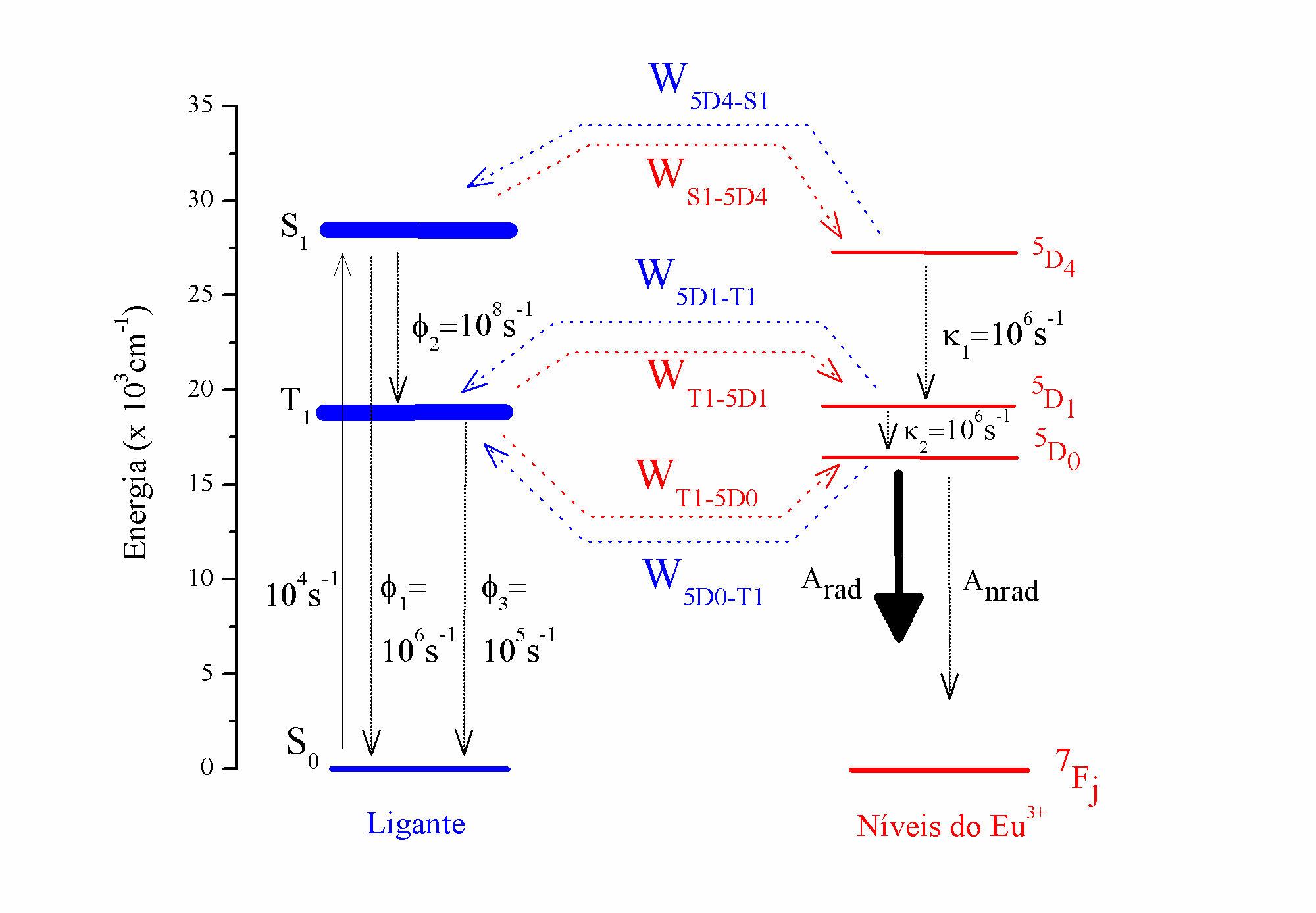
Figure 2. Transfer channels involved in the energy transfer rate processes of systems containing europium ion.

The total angular momentum selection rules, $J$ , of the lanthanide 4f states, are complementary. The europium excited states that are more likely to accept energy from ligands through the direct Coulomb interaction mechanism are ⁵D₂, ⁵L₆, ⁵G₆, and ⁵D₄. The energy transfer from ligand excited states to the ⁵D₁ level is allowed by the exchange interaction mechanism (Eq. ( $\ref{eq:wet_em}$ )). Although the energy transfer to the ⁵D₀ level, in principle, is forbidden by direct interaction or exchange mechanism, the selection rule can be relaxed by a mix of the total angular moments ( $J$ ’s) [43, 45].

Emission Quantum Yield Calculation

The emission quantum yield, given by Eq. ( $\ref{eq:q}$ ), is defined as the ratio between the emitted and absorbed light intensities.

q=\frac{{{A}_{rad}}{{\eta }_{{}^{5}{{D}_{0}}}}}{\varphi \eta {}_{{{S}_{0}}}} \label{eq:q}

where ${{\eta }_{{}^{5}{{D}_{0}}}}$ is the ⁵D₀ level population. $\eta {}_{{{S}_{0}}}$ and $\varphi$ correspond to the S₀ singlet level population and absorption rate, respectively. The normalized population levels, $\eta_j$ , are obtained from the appropriate rate equations given by Eq. ( $\ref{eq:q}$ ).

\frac{d{{\eta }_{j}}}{dt}=-\left( \sum\limits_{i\ne j}{{{W}_{ji}}} \right){{\eta }_{j}}+\sum\limits_{i\ne j}{{{W}_{ij}}}{{\eta }_{i}} \label{eq:eta}

From Eq. ( $\ref{eq:q}$ ), $W_{ij}$ or $W_{ji}$ represent the transfer rates between $i$ and $j$ states, or $j$ and $i$ states.

The ⁵D₀ level population depends on the non-radiative emission rate $A_{nrad}$ , which still cannot be theoretically calculated. However, $A_{nrad}$ can be quantified via Eq. ( $\ref{eq:tau}$ ) from the $A_{rad}$ and the experimental lifetime ( $\tau$ ). Because of this, the theoretical emission quantum yield depends on the experimental lifetime.

\frac{1}{\tau }={{A}_{rad}}+{{A}_{nrad}} \label{eq:tau}

The normalized populations of the states involved in the process of energy transfer are obtained from diagonalizing the matrix that contains the rate equations showed in Figure 3. As can been in Figure 3, the matrix is assembled from energy transfer and back-transfer rates, $A_{rad}$ and $A_{nrad}$ . The matrix diagonal contains the transfer channels responsible for the energy depopulation of the states in the matrix columns. The channels in red (Figure 2) are not normally included in the energy transfer rates diagrams (Figure 2) due to the non-resonance condition presented between some ligand and the europium excited states.

The emission quantum yield is then calculated from the population given by Eq. ( $\ref{eq:q}$ ).

	S₀	Singlet	Triplet	⁵D₄	⁵D₁	⁵D₀
	1	1	1	1	1	1
Singlet	10⁴	$-[(W_{S-{^5}D_4}+\phi_1+\\ \phi_2+\textcolor{red}{W_{S-^5D_1}} +\\ \textcolor{red}{W_{S-{^5}D_0}})]$	0	$W_{^5D_4-S}$	$\textcolor{red}{W_{^5D_1-S}}$	$\textcolor{red}{W_{^5D_0-S}}$
Triplet	0	$\phi_2$	$-(W_{T-^5D_1}+\\W_{T-5D0}+\phi_3+\\ \textcolor{red}{W_{T-^5D_4}})$	$\textcolor{red}{W_{^5D_4-T}}$	$W_{^5D_1-T}$	$W_{^5D_0-T}$
⁵D₄	0	$W_{S-^5D_4}$	$\textcolor{red}{W_{T-^5D_4}}$	$-[(W_{^5D_4-S}+\\k_1+\textcolor{red}{W_{^5D_4-T}})]$	0	0
⁵D₁	0	$\textcolor{red}{W_{S-^5D_1}}$	$W_{T-5D_1}$	$k_1$	$-[(W_{^5D_1-T}+\\k_2+\textcolor{red}{W_{^5D_1-S}})]$	0
⁵D₀	0	$\textcolor{red}{W_{S-^5D_0}}$	$W_{T-^5D_0}$	0	$k_2$	$-[(\textcolor{red}{W_{^5D_0-S}}+\\ W_{^5D_0-T}+\\A_{rad}+A_{nrad})]$

Figure 3. Matrix for obtaining the normalized energy level population, enabling the theoretical calculation of the emission quantum yield.

Bibliographic References

[1] Lewars, E.G., Computational Chemistry: Introduction to the Theory and Applications of Molecular and Quantum Mechanics2010: Springer.

[2] Freire, R.O., G.B. Rocha, and A.M. Simas, Lanthanide complex coordination polyhedron geometry prediction accuracies of ab initio effective core potential calculations. Journal of Molecular Modeling, 2006. 12(4): p. 373-389.

[3] Rodrigues, D.A., N.B. da Costa, and R.O. Freire, Would the Pseudocoordination Centre Method Be Appropriate To Describe the Geometries of Lanthanide Complexes? Journal of Chemical Information and Modeling, 2011. 51(1): p. 45-51.

[4] de Andrade, A.V.M., et al., Sparkle Model for the Quantum-Chemical Am1 Calculation of Europium Complexes. Chemical Physics Letters, 1994. 227(3): p. 349-353.

[5] Rocha, G.B., et al., Sparkle Model for AM1 Calculation of Lanthanide Complexes: Improved Parameters for Europium. Inorganic Chemistry, 2004. 43(7): p. 2346-2354.

[6] Freire, R.O., G.B. Rocha, and A.M. Simas, Sparkle model for the calculation of lanthanide complexes: AM1 parameters for Eu(III), Gd(III), and Tb(III). Inorganic Chemistry, 2005. 44(9): p. 3299-3310.

[7] da Costa, N.B., et al., Sparkle/AM1 modeling of holmium (III) complexes. Polyhedron, 2005. 24(18): p. 3046-3051.

[8] Freire, R.O., G.B. Rocha, and A.M. Simas, Modeling lanthanide complexes: Sparkle/AM1 parameters for ytterbium (III). Journal of Computational Chemistry, 2005. 26(14): p. 1524-1528.

[9] Freire, R.O., et al., Modeling lanthanide coordination compounds: Sparkle/AM1 parameters for praseodymium (III). Journal of Organometallic Chemistry, 2005. 690(18): p. 4099-4102.

[10] da Costa, N.B., et al., Sparkle model for the AM1 calculation of dysprosium (III) complexes. Inorganic Chemistry Communications, 2005. 8(9): p. 831-835.

[11] Freire, R.O., G.B. Rocha, and A.M. Simas, Modeling rare earth complexes: Sparkle/AM1 parameters for thulium (III). Chemical Physics Letters, 2005. 411(1-3): p. 61-65.

[12] Freire, R.O., et al., AM1 sparkle modeling of Er(III) and Ce(III) coordination compounds. Journal of Organometallic Chemistry, 2006. 691(11): p. 2584-2588.

[13] Freire, R.O., et al., Sparkle/AM1 structure modeling of lanthanum (III) and lutetium (III) complexes. Journal of Physical Chemistry A, 2006. 110(17): p. 5897-5900.

[14] Freire, R.O., et al., Sparkle/AM1 parameters for the modeling of samarium(III) and promethium(III) complexes. Journal of Chemical Theory and Computation, 2006. 2(1): p. 64-74.

[15] Freire, R.O., G.B. Rocha, and A.M. Simas, Modeling rare earth complexes: Sparkle/PM3 parameters for thulium(III). Chemical Physics Letters, 2006. 425(1-3): p. 138-141.

[16] Freire, R.O., et al., Sparkle/PM3 parameters for the modeling of neodymium(III), promethium(III), and samarium(III) complexes. Journal of Chemical Theory and Computation, 2007. 3(4): p. 1588-1596.

[17] Freire, R.O., G.B. Rocha, and A.M. Simas, Sparkle/PM3 parameters for praseodymium(III) and ytterbium(III). Chemical Physics Letters, 2007. 441(4-6): p. 354-357.

[18] da Costa, N.B., et al., Structure modeling of trivalent lanthanum and lutetium complexes: Sparkle/PM3. Journal of Physical Chemistry A, 2007. 111(23): p. 5015-5018.

[19] Simas, A.M., R.O. Freire, and G.B. Rocha, Cerium (III) complexes modeling with Sparkle/PM3. Computational Science - Iccs 2007, Pt 2, Proceedings, 2007. 4488: p. 312-318.

[20] Simas, A.M., R.O. Freire, and G.B. Rocha, Lanthanide coordination compounds modeling: Sparkle/PM3 parameters for dysprosium (III), holmium (III) and erbium (III). Journal of Organometallic Chemistry, 2008. 693(10): p. 1952-1956.

[21] Freire, R.O., G.B. Rocha, and A.M. Simas, Sparkle/PM3 for the Modeling of Europium(III), Gadolinium(III), and Terbium(III) Complexes. Journal of the Brazilian Chemical Society, 2009. 20(9): p. 1638-1645.

[22] Freire, R.O. and A.M. Simas, Sparkle/PM6 Parameters for all Lanthanide Trications from La(III) to Lu(III). Journal of Chemical Theory and Computation, 2010. 6(7): p. 2019-2023.

[23] Dutra, J.D.L., et al., Sparkle/PM7 Lanthanide Parameters for the Modeling of Complexes and Materials. Journal of Chemical Theory and Computation, 2013. 9(8): p. 3333-3341.

[24] Filho, M.A.M., et al., Sparkle/RM1 parameters for the semiempirical quantum chemical calculation of lanthanide complexes. RSC Advances, 2013. 3(37): p. 16747-16755.

[25] Stewart, J.J.P., MOPAC2009, 2009, Colorado Springs: USA. p. Stewart Computational Chemistry.

[26] Stratmann, R.E., G.E. Scuseria, and M.J. Frisch, An efficient implementation of time-dependent density-functional theory for the calculation of excitation energies of large molecules. Journal of Chemical Physics, 1998. 109(19): p. 8218-8224.

[27] Ridley, J.E. and M.C. Zerner, Triplet-States Via Intermediate Neglect of Differential Overlap - Benzene, Pyridine and Diazines. Theoretica Chimica Acta, 1976. 42(3): p. 223-236.

[28] Zerner, M.C., et al., Intermediate Neglect of Differential-Overlap Technique for Spectroscopy of Transition-Metal Complexes - Ferrocene. Journal of the American Chemical Society, 1980. 102(2): p. 589-599.

[29] Santos, J.G., et al., Theoretical Spectroscopic Study of Europium Tris(bipyridine) Cryptates. Journal of Physical Chemistry A, 2012. 116(17): p. 4318-4322.

[30] Zerner, M.C., ZINDO manual QTP, 1990, University of Florida: Gainesville.

[31] Neese, F., The ORCA program system. Wiley Interdisciplinary Reviews-Computational Molecular Science, 2012. 2(1): p. 73-78.

[32] de Andrade, A.V.M., et al., Theoretical model for the prediction of electronic spectra of lanthanide complexes. Journal of the Chemical Society-Faraday Transactions, 1996. 92(11): p. 1835-1839.

[33] Judd, B.R., Optical Absorption Intensities of Rare-Earth Ions. Physical Review, 1962. 127(3): p. 750-&.

[34] Ofelt, G.S., Intensities of Crystal Spectra of Rare-Earth Ions. Journal of Chemical Physics, 1962. 37(3): p. 511-&.

[35] Freeman, A.J. and J.P. Desclaux, Dirac-Fock Studies of Some Electronic Properties of Rare-Earth Ions. Journal of Magnetism and Magnetic Materials, 1979. 12(1): p. 11-21.

[36] Malta, O.L., et al., Theoretical Intensities of 4f-4f Transitions between Stark Levels of the Eu3+ Ion in Crystals. Journal of Physics and Chemistry of Solids, 1991. 52(4): p. 587-593.

[37] Mason, S.F., R.D. Peacock, and B. Stewart, Dynamic coupling contributions to the intensity of hypersensitive lanthanide transitions. Chemical Physics Letters, 1974. 29(2): p. 149-153.

[38] Malta, O.L., A Simple Overlap Model in Lanthanide Crystal-Field Theory. Chemical Physics Letters, 1982. 87(1): p. 27-29.

[39] Malta, O.L., Theoretical Crystal-Field Parameters for the Yoc1 - Eu-3+ System - a Simple Overlap Model. Chemical Physics Letters, 1982. 88(3): p. 353-356.

[40] Carnall, W.T., H. Crosswhite, and H.M. Crosswhite, Energy level structure and transition probabilities of the trivalent lanthanides in LaF3, 1977: Argonne National Laboratory.

[41] Peacock, R., The intensities of lanthanide f ↔ f transitions, in Rare Earths 1975, Springer Berlin Heidelberg. p. 83-122.

[42] Malta, O.L., Ligand-rare-earth ion energy transfer in coordination compounds. A theoretical approach. Journal of Luminescence, 1997. 71(3): p. 229-236.

[43] Silva, F.R.G.E. and O.L. Malta, Calculation of the ligand-lanthanide ion energy transfer rate in coordination compounds: Contributions of exchange interactions. Journal of Alloys and Compounds, 1997. 250(1-2): p. 427-430.

[44] Malta, O.L., Mechanisms of non-radiative energy transfer involving lanthanide ions revisited. Journal of Non-Crystalline Solids, 2008. 354(42-44): p. 4770-4776.

[45] de Sa, G.F., et al., Spectroscopic properties and design of highly luminescent lanthanide coordination complexes. Coordination Chemistry Reviews, 2000. 196: p. 165-195.